Locating Factual Knowledge in GPT-2

This example shows how to use Inseq to locate factual knowledge in GPT-2, adopting the contrastive attribution method described in “Interpreting Language Models with Contrastive Explanations” by Yin and Neubig (2022).

Thanks to bitsandbytes integration, we can attribute the GPT-2 XL model (1.5B parameters) using the layer_gradient_x_activation method on very affordable hardware (tested on a 6GB Nvidia RTX 3060 GPU). The following code snippet loads the model and runs attribution for intermediate layers of the model on the whole Counterfact Tracing dataset by Meng et al. (2022), saving aggregated outputs to disk.

import inseq
from datasets import load_dataset
from transformers import AutoModelForCausalLM, AutoTokenizer

# The model is loaded in 8-bit on available GPUs
model = AutoModelForCausalLM.from_pretrained("gpt2-xl", load_in_8bit=True, device_map="auto")
tokenizer = AutoTokenizer.from_pretrained("gpt2-xl")
# Counterfact datasets used by Meng et al. (2022)
data = load_dataset("NeelNanda/counterfact-tracing")["train"]

# GPT-2 XL is a Transformer model with 48 layers
for layer in range(48):
    attrib_model = inseq.load_model(
        model,
        "layer_gradient_x_activation",
        tokenizer="gpt2-xl",
        target_layer=model.transformer.h[layer].mlp,
    )
    for i, ex in data:
        # e.g. "The capital of Spain is"
        prompt = ex["relation"].format(ex["subject"])
        # e.g. "The capital of Spain is Madrid"
        true_answer = prompt + ex["target_true"]
        # e.g. "The capital of Spain is Paris"
        false_answer = prompt + ex["target_false"]
        # Contrastive attribution of true vs false answer
        out = attrib_model.attribute(
            prompt,
            true_answer,
            attributed_fn="contrast_prob_diff",
            contrast_targets=false_answer,
            step_scores=["contrast_prob_diff"],
            show_progress=False,
        )
        # Save aggregated attributions to disk
        out = out.aggregate()
        out.save(f"layer_{layer}_ex_{i}.json", overwrite=True)

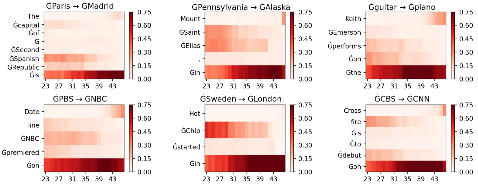
The following plots visualize attributions per layers for some examples taken from the dataset, showing how intermediate layers play a relevant role in recalling factual knowledge, in relation to the last subject token in the input: